What O(n) actually promises

Every problem page on this site ends with a line that says “Aim for O(n) time” or “Aim for O(n log n)”. The notation looks like a score, but it is not clear what it measures. Is O(n log n) a good grade or a bad one? This article explains what the notation promises, how to read it, and why the input size on a problem page is the most useful clue to the algorithm the problem expects.

The promise is about growth, not speed

O(n) does not tell you how many milliseconds an algorithm takes. It tells you how the work grows as the input grows. An algorithm that is O(n) does work in proportion to the input: double the input, double the work. An algorithm that is O(n^2) does work proportional to the square: double the input, quadruple the work. The O stands for “order of”, and the expression inside the parentheses describes the growth curve, not a runtime.

That is why constants do not appear in the notation. An algorithm that does 3n + 7 units of work and one that does 100n + 2 are both O(n), because the constant multipliers and offsets disappear next to the shape. The notation is coarse by design. It compares growth classes, not individual runs. On small inputs, that comparison can mislead: an O(n^2) algorithm with tiny constants can beat an O(n log n) one on an input of size ten. Big-O does not care. It describes what happens as the input gets large, which is where algorithms live or die.

The ladder

The growth classes you meet on this site, in order:

• O(1) - constant work: the same no matter the input. Reading one element of an array, looking up a hash key.
• O(log n) - work grows slowly: binary search, which halves the remaining input each step.
• O(n) - one pass over the input: scanning a list, or the map and filter shapes from the refactoring exercises.
• O(n log n) - the dividing-and-recombining algorithms: most good sorts. The log factor is the price of the repeated halving.
• O(n^2) - the nested loops: comparing every pair, or the loops you meet early in the refactoring exercises before they become map and filter.

The ladder gives you the vocabulary. When a problem says “Aim for O(n)” and your first idea is a nested loop that scans the list once per element, the notation tells you that loop has the wrong shape. It is O(n^2). The same job can be done in one pass, usually by remembering something about the elements you have already seen.

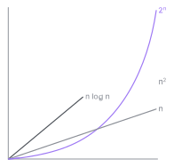
The shapes are the point. Look at them instead of trying to picture them. The same input size can produce wildly different amounts of work, and the difference compounds as the curves suggest. Linear work and exponential work are not “a bit apart”. They are different universes that happen to look adjacent at n = 10.

The input size is the hint

This is the practical skill the notation gives you. The problem page provides the input’s size limits, and those limits rule out entire families of algorithms. A list with up to a hundred thousand elements cannot be handled by an O(n^2) algorithm - ten billion operations - so the problem is pointing toward O(n) or O(n log n). A problem capped at twenty elements points the other way: an exponential search over subsets is affordable, and the intended solution may genuinely be brute force or a bitmask over the elements. The size limit is not a footnote. It tells you which growth class the problem expects before you read a word about the algorithm.

Read a problem in two steps: look at the size limits, pick the growth class they permit, then find the technique that lands in that class. Sorting is O(n log n); a scan with a hash map is O(n); a binary search over a sorted range is O(log n) per probe. When the size limits say “a hundred thousand”, the answer is almost never the nested loop.

What the notation does not promise

Big-O is a bound on work, not a guarantee about your program. It says nothing about the constant factor, so an O(n) algorithm can be slower than an O(n log n) one on the inputs you actually have. A factor of ten separates a demo from a product, and the notation cannot see it. It says nothing about memory unless the problem says so. “O(n) time, O(n) memory” is two promises, and the second one can be the binding constraint. Big-O also describes the worst case (or the average, depending on the algorithm), not every run: a sort that is O(n log n) on average can still degrade. The notation is a contract about growth, and the problems on this site use it that way: “Aim for O(n)” makes a claim about the solution’s shape. Check it by asking whether your algorithm makes one pass or nested passes over the input.

Why this matters here

The complexity budget is the second sentence of every problem description, after the goal. The memory cards and problem cards carry the labels; the algorithm-approach articles show a solver naming the growth class before writing the code. Read the notation and turn “I need to solve this problem” into “I need a one-pass solution, so I should remember what I have seen rather than re-scan it.” The size limit gives away the problem’s difficulty class. The notation makes that hint legible.

Where to go next

• Sorting: the wall at n log n - the $n \log n$ shape, earned one comparison at a time, and the wall that no comparison sort can cross.
• Hash tables: the O(1) that has fine print
  • what “O(1) on average” actually promises, load factor and collisions included.
• Dynamic programming: recursion with a cache
  • the shape change from $2^n$ to $n$, the same contract in its most dramatic register.
• Graphs: when the answer is a hop away
  • $O(V + E)$: the shape of a graph walk, where the size of the graph is the honest input size.
• Dijkstra’s algorithm: when every hop costs something
  • $O((V + E) \log V)$: the priority queue that buys the log, and the constant factor that decides which sort wins.
• Binary trees: where the log in O(log n) lives
  • the doubling argument, and where the log in all of the above lives.
• P vs NP: when a thousand cores won’t help
  • the other side of the same contract: the shape no algorithm can have.