Sorting: the wall at n log n

Every algorithm practice path starts with sorting. It is the problem in every textbook, the implementation every candidate gets asked for, and the exercise this site grades in four languages at once - the Merge Sort exercise in /problems runs the same input through the Elixir, Erlang, TypeScript, and Lua runners. Sorting earns that place for a harder reason than simplicity. It is where the limits begin: a wall at $n \log n$ that no comparison-based sorting algorithm can cross. This article gets there through simple sorts, divide-and-conquer sorts, and the proof that no comparison sort can keep improving forever.

The problem and the obvious answer

The sorting problem needs no ceremony. The algorithms textbook opens its sorting chapter with it: “Given an array of unsorted values, how can we sort them so that they end up in ascending order?” That is the specification. The obvious implementation uses nested loops: walk the list, find the smallest remaining element, swap it into place, and repeat. The textbook puts these algorithms in the right family:

Some of the first ones you’ll learn about are known as simple sorts, in that they are easy to understand but are not as efficient as some of the faster sorting algorithms out there.

“Easy to understand” is only half the story. Count the comparisons. Selection sort - find the minimum, put it first, repeat on the rest - makes exactly $n(n-1)/2$ comparisons: the first pass scans all $n$ elements, the second scans $n-1$, and so on. The textbook works through five elements: the first pass makes four comparisons, the second makes three, “because we didn’t have to compare the final two numbers, since we knew that the final number was in the correct spot.” Four plus three plus two plus one is ten, which is $5 \cdot 4 / 2$.

The nested loop’s shape appears in the arithmetic. Ten elements cost 45 comparisons; a hundred cost 4,950; a million cost 499,999,500,000 - about half a trillion. The list does not need to be huge. A million elements fits in a text file, a database table, or a column of log lines. Half a trillion operations is still half a trillion operations. This is the quadratic cliff, the shape this site’s What O(n) actually promises article warns about: $O(n^2)$ means the work grows with the square of the input, and doubling the input quadruples the work, forever.

Merge sort: divide and conquer

The way past the quadratic cliff is simple: stop repeating work. Merge sort splits a list in half, sorts each half recursively, and merges the two sorted halves into one sorted whole. One-element lists end the recursion because they are sorted by definition. The merge step does the work: walk two sorted lists, compare their fronts, and emit the smaller one - at most $n$ comparisons per merge.

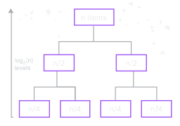
Count the merges. Splitting a list in half, then in half again, creates about $\log_2 n$ levels of recursion - a million elements split into two, then four, then eight, … until singletons, which takes about twenty levels. Each level merges lists with total size $n$, because every element is merged once at that level. Each level therefore costs about $n$ comparisons. The total is $n \log_2 n$: for a million elements, about twenty million comparisons instead of half a trillion - roughly twenty-five thousand times fewer. The gap grows with the list.

Name the analysis technique. It has the same shape as the site’s Induction content. The algorithms textbook counts with a recursion tree: “We’ll analyze MergeSort using the ‘recursion tree method,’ which is a way of tallying up the operations performed by a recursive algorithm.” Draw the recursion as a tree: the root splits the full list and the leaves are singletons. The tree has $\log_2 n$ levels, each with a constant $n$ worth of work. A recursive algorithm’s cost is the sum of that tree. This is the induction argument in asymptotic notation, and it is why this site’s binary trees article - where the log in $O(\log n)$ lives - belongs next to sorting. The merge tree is a binary tree. The log was already there.

The site’s Merge Sort exercise asks for exactly this: implement merge_sort, and the grader runs it against hidden cases in all four runners. If you solved the Recursion exercises, the structure should look familiar. The function calls itself on smaller inputs and trusts the recursion to do the work. That is the inductive hypothesis at the heart of Induction.

Quicksort: the rival

Merge sort is not the only divide-and-conquer sort, and it is not the sort you will meet most often in practice. Quicksort - the subject of a whole chapter in the standard algorithms introduction - takes a different route: it splits by value and does the work in the partition. Pick a pivot, rearrange the list so everything smaller than the pivot is on one side and everything larger is on the other, then recurse on both sides. There is no merge step. The partition puts the pivot in its final position, and the recursive calls sort around it.

The introduction states its place in the complexity hierarchy plainly: “$O(n \cdot \log n)$. Example: a fast sorting algorithm, like quicksort.” The qualification is in the word “average.” Quicksort’s partitioning pays off when the pivot splits the list into roughly equal halves. If the pivot is always the smallest (or largest) element - which happens when you pick the first element and the list is already sorted, the classic worst case - one side of every partition is empty, the recursion tree becomes a chain, and the cost returns to the quadratic cliff. Merge sort has no such failure mode. Its splits are by position, not by value, so they stay balanced whatever the data looks like. Its worst case is $O(n \log n)$, guaranteed.

The introduction asks the obvious question verbatim: “If quicksort is $O(n \log n)$ on average, but merge sort is $O(n \log n)$ always, why not use merge sort? Isn’t it faster?” The answer is the part big O hides: the constant factor. Both grow like $n \log n$, but quicksort’s average constant is smaller. In-place partitioning touches fewer elements and moves less data than merging into a fresh list. Its locality is also friendlier to the memory hierarchy this site’s stored-program article spent its middle section on. Big O describes the curve’s shape, not its height; two algorithms with the same big O can differ by a factor of ten in wall-clock time. The What O(n) article makes the same point: the notation promises the shape, and nothing else.

Production sorting chooses between these tradeoffs. Python’s sort and JavaScript’s sort use Timsort, a hybrid of merge sort and insertion sort that exploits already-sorted runs in the input.timsort Erlang’s lists:sort - the sort under Elixir’s Enum.sort - is a merge sort, tuned for the constant factor: merging suits the immutable linked lists that are the only list in Elixir, and the recursion runs well on the BEAM.erlang-sort Do not reduce the choice to “merge sort beats quicksort” or the reverse. The analysis gives you the shape of the contest; the constant factor decides the details. That is why the same problem graded by this site’s runners in four languages is genuinely four different programs.

The wall: why n log n is the floor

Both merge sort and quicksort sit at $n \log n$. What comes after? Is there an $O(n)$ comparison sort nobody has found yet? No. The answer comes from information theory, not from trying harder. That is why sorting is taught alongside the halting problem in every theory course: both are limits, not failures of imagination.

A comparison-based sort is a decision tree. Every comparison asks a yes/no question - “is this element smaller than that one?” - and the answers determine which ordering the sort outputs. There are $n!$ possible orderings of $n$ distinct elements, and the sort must distinguish all of them because any one could be the input. A yes/no comparison carries at most one bit of information: it can cut the candidate orderings in half at best. Distinguishing $n!$ orderings therefore requires at least $\log_2(n!)$ comparisons in the worst case.knuth-taocp Stirling’s approximation says $\log_2(n!)$ grows like $n \log_2 n$ minus a small linear term. No comparison sort can do better.clrs-sorting The information has to come from somewhere, and each comparison supplies one bit.

The wall is not a technology limit. A faster machine, a cleverer compiler, or a bigger cache cannot move it, just as a thousand cores cannot fix an exponential algorithm in this site’s P vs NP article. This is an information limit: the order was not in the bytes, so the sort has to earn it, one bit per comparison. That is the point made by the bits-have-no-meaning argument: the bits of an unsorted list carry no inherent order, and extracting that order is measured, not invented.

The exception makes the rule clear. Sorting algorithms that do not use comparisons - counting sort, radix sort - can reach $O(n)$ by using the values as array indices.clrs-sorting If every key is a small integer, “sort” becomes “tally how many of each value there are and emit them in order,” which is not comparison at all. The wall binds only the comparison family. Once the algorithm stops asking yes/no questions about elements and starts using what the elements are, different and stricter assumptions about the input allow a different curve.

Where the wall meets practice

The practical takeaway is already built into the site’s exercises. When you write Enum.sort, you are using a tuned merge sort. When a coding interview asks for a sort, the interviewer usually wants to know which family you are in and what the wall says about it. Do not memorize three algorithms in isolation. Read the shape: nested loops over the whole list are quadratic, splitting-and-merging is $n \log n$, and any claim of a faster comparison sort is either wrong or limited to a restricted input. Name the curve, then choose the implementation. That is the same move this site’s Algorithms past the interview article identifies as the heart of the handshake: name the bound before the incident does it for you.

Where to go next

• Merge Sort on /problems - implement merge_sort and watch the same algorithm run in four languages.
• Merge Sorted Lists - the merge step of merge sort, extracted into its own exercise; the piece that does the real work.
• Binary trees: where the log in O(log n) lives
  • the tree whose height is the log; the merge tree is that shape.
• What O(n) actually promises - the shape-vs-constant distinction that decides merge sort against quicksort.
• Recursion and Induction - the machinery merge sort is made of: a function that calls itself and a proof that the call is the hypothesis.
• Bits have no meaning and The halting problem
  • the limits family sorting’s wall belongs to: information limits and decision limits, neither movable by hardware.

Sorting is where the depth starts because it exposes the limits. Simple sorts teach the quadratic cliff. Merge sort teaches the recursive pattern that escapes it. The wall at $n \log n$ explains why that escape cannot continue: the order was never in the bytes, and every comparison earns one bit of it. That is algorithmic thinking in one problem: recognize the shape, choose the structure, and know which wall stands in front of you.