Dijkstra's algorithm: when every hop costs something

The previous article in this pair - Graphs: when the answer is a hop away - ended with a promise. Breadth-first search finds the shortest path in hops, but real maps price roads by time, distance, or cost. A drive across town and a drive around town can use the same number of edges and take very different amounts of time. Once edges carry prices, “shortest path” means “cheapest route,” not “fewest hops.” The algorithm changes too. That algorithm is Dijkstra’s algorithm, named after Edsger Dijkstra, who published it in

1959. It is one of the most-used algorithms in existence: every navigation system, every network router, every package tracker runs a version of it. Dijkstra said he designed the algorithm in about twenty minutes in 1956, sitting with his fiancée on a café terrace in Amsterdam. He had no pen and paper, so he worked out the entire design in his head. It is a rare algorithm with a café in its origin story instead of a whiteboard. It has run navigation systems ever since. This article covers the problem it solves, the four-step method, a worked example you can trace by hand, and the limits that keep it from solving every shortest-path problem.

The problem: when every hop costs something

The graphs article introduced the two-part model - nodes and edges - and the rule that decides which algorithm applies. The algorithms introduction states it exactly:

A graph with weights is called a weighted graph. A graph without weights is called an unweighted graph.

The resulting rule is the whole decision procedure:

To calculate the shortest path in an unweighted graph, use breadth-first search. To calculate the shortest path in a weighted graph, use Dijkstra’s algorithm.

BFS stops working when weights appear because BFS measures a path in hops. Hops are no longer what you want to minimize. Here is a small graph you can hold in your head: from start A, a road to C costs 2 and a road to B costs 4; from C, a road to B costs 1 and a road to D costs 5; from B, a road to D costs 1. The cheapest route from A to D takes three hops - A to C to B to D, at 2 + 1 + 1 = 4. The two-hop routes cost more: A to B to D costs 4 + 1 = 5, and A to C to D costs 2 + 5 = 7. BFS counts hops, so it would call the 5-cost two-hop route “shorter” than the 4-cost three-hop route. Fewest hops and cheapest route have split apart. This is a weighted-graph problem.

The four steps

Dijkstra’s algorithm is simple to state. The introduction’s version fits in four steps, and the first two contain the main idea:

1. Find the cheapest node. This is the node you can get to in the least amount of time.
2. Check whether there’s a cheaper path to the out-neighbors of this node. If so, update their costs.

The reference treatment gives the formal version: “Dijkstra proposed an iterative algorithm to find shortest distances from a single source.” That is the contract: one source, with the shortest distance to every reachable node as the result. The machinery is two small structures. A distance table stores the cheapest known cost for every node, starting at 0 for the source and infinity for everyone else. A settled set stores the nodes whose distance is final - the nodes the algorithm has committed to. The loop repeats the two steps above: pick the cheapest unsettled node, then relax its edges. For each out-neighbor, ask “is the cost through this node less than what the table currently says?” If it is, update the table. When every node is settled, the table is the answer.

The word “relax” matters because it names the entire algorithm. Relaxing an edge compares two candidate routes to a node: the known route and the route through the current node. Keep the cheaper one. That is all the algorithm does. It relaxes edges in the order set by the cheapest-first frontier, and that order guarantees the result is the best route, not just a good one.

A worked example

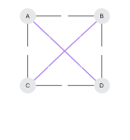
Run the four steps on the graph from the problem section. Write distances as node: cost and the settled set in braces. Keep the graph in sight as you trace it. The cheapest route is three hops (2 + 1 + 1), while both two-hop routes cost more:

Start: table {A: 0, B: inf, C: inf, D: inf}, settled {}.

• Step 1, settle A (0). Relax A’s edges: B is reachable at 4, C at 2. Table {A: 0, B: 4, C: 2, D: inf}, settled {A}.
• Step 2, settle C (2) - C is the cheapest unsettled node. Relax C’s edges: B is reachable at 2 + 1 = 3, and 3 is cheaper than the table’s 4, so B drops to 3. D is reachable at 2 + 5 = 7. Table {A: 0, B: 3, C: 2, D: 7}, settled {A, C}.
• Step 3, settle B (3) - cheaper than D’s 7. Relax B’s edge: D is reachable at 3 + 1 = 4, cheaper than the table’s 7, so D drops to 4. Table {A: 0, B: 3, C: 2, D: 4}, settled {A, C, B}.
• Step 4, settle D (4). D has no out-edges. Table {A: 0, B: 3, C: 2, D: 4}, settled {A, C, B, D}. Done.

Stop at Step 2 and look closely. The table first said B was reachable at 4 through the direct road A to B. Settling C exposed a cheaper route, A to C to B at 3, so the algorithm updated the table. It repeats that update across the graph. That is why the final table gives the cheapest route, not merely a route: each distance comes from asking, node by node, “is there a cheaper way through the node I just settled?” The final table says the cheapest way to D costs 4, via C and B - the three-hop route that beat both two-hop routes.

The algorithm in code

The same four steps take a few lines in a functional language. Read the shape: a pure function threads an immutable distance table, with no mutation and no hidden state. That is the site’s philosophy in miniature, and it is the same discipline the Substitutions and Functions exercises teach, applied to a classic imperative algorithm.

defmodule Dijkstra do
  def shortest(graph, start) do
    do_shortest(graph, %{start => 0}, MapSet.new())
  end

  defp do_shortest(graph, dist, settled) do
    case Enum.reject(dist, fn {n, _} -> MapSet.member?(settled, n) end) do
      [] ->
        dist

      frontier ->
        {node, cost} = Enum.min_by(frontier, fn {_n, c} -> c end)

        new_dist =
          Enum.reduce(Map.get(graph, node, []), dist, fn {nb, w}, acc ->
            if cost + w < Map.get(acc, nb, :infinity) do
              Map.put(acc, nb, cost + w)
            else
              acc
            end
          end)

        do_shortest(graph, new_dist, MapSet.put(settled, node))
    end
  end
end

Run it on the worked example - graph with a at 0 and edges a->b: 4, a->c: 2, c->b: 1, c->d: 5, b->d: 1 - and it returns %{a: 0, c: 2, b: 3, d: 4}, the exact table from the hand trace. The recursion is the loop. The case on the frontier is the “pick the cheapest unsettled node” step. The reduce performs the relaxation. The function keeps a frontier of known distances, commits to the cheapest node, and lets that commitment improve every node it can reach.

Why the frontier is a priority queue

The deciding step - “find the cheapest unsettled node” - determines the algorithm’s data structure. The version above scans the whole distance table on every iteration, which makes it $O(V^2)$ on a graph with $V$ nodes: for each of the $V$ settled nodes, it scans up to $V$ candidates. A production version replaces that scan with a priority queue, a structure that returns the minimum element in $O(\log n)$ instead of $O(n)$. A priority queue is usually a heap. A binary heap is a binary tree arranged so the smallest element sits at the root - the tree shape from the site’s binary trees article, doing the same job the log always does. With a heap holding the frontier, Dijkstra runs in $O((V + E) \log V)$ where $E$ is the number of edges: each node is extracted once, each edge is relaxed once, and each heap operation costs the log. The formulas describe the same algorithm. The heap separates the version that scales from the version that teaches.

The fine print: greedy commitments and negative weights

Dijkstra works because it makes one commitment, and that commitment sets its boundary. When the algorithm settles a node - commits its distance as final - it assumes no later discovery can produce a cheaper route to that node. This is a greedy choice: at every step, take the locally cheapest frontier node and never look back. The choice is sound for non-negative weights. Any alternative route to a settled node would have to pass through an unsettled node, and every unsettled node is at least as far away as the one just settled, so that route can only cost more. The graph-algorithms reference states the guarantee as a theorem: “for each vertex in the settled set at any time during Dijkstra’s [execution], its distance is final.”

The limit is the word “non-negative.” The algorithms introduction warns in its summary: “You learn about negative-weight edges in graphs, where Dijkstra’s algorithm doesn’t work.” The failure comes from the commitment. Suppose A to B costs 2 and A to C costs 5, but C to B costs -4 - a road that refunds you for taking it. Dijkstra settles B at 2, the cheapest unsettled node, before it visits C. When C is later settled and the edge C to B is relaxed, the true route A to C to B at 5 - 4 = 1 appears - but B is already settled, and the algorithm cannot revise that commitment. The greedy assumption was that no later route could be cheaper. A negative edge is exactly such a later route. For graphs with negative weights, use the Bellman-Ford algorithm, which relaxes every edge in rounds and permits the revision Dijkstra forbids. The moral is the one this site’s What O(n) article teaches about every complexity claim: the guarantee holds under stated assumptions, and naming those assumptions is part of using the algorithm.

Where Dijkstra lives

Dijkstra’s algorithm is the weighted-graph answer to the graphs article’s unweighted one: BFS when every hop costs the same, Dijkstra when it does not, Bellman-Ford when weights can go negative. The site’s exercise catalog does not yet have a weighted-graph problem. The graphs exercise, Number of Islands, is an unweighted connected-components problem, and Process Ring is an unweighted cycle. This article, like the graphs article, is the theory half of a feature that would complete it: a seeded weighted-graph exercise paired with the priority-queue data structure the algorithm’s frontier needs. The site already has the pieces: the queue from the data-structures article, the log from the binary trees article, and the greedy analysis in this article’s worked example.

Where to go next

• Graphs: when the answer is a hop away
  • the unweighted half: BFS, connected components, and the graph model this article assumes.
• Number of Islands and Process Ring - the site’s existing graph exercises, both unweighted.
• Binary trees: where the log in O(log n) lives
  • the heap is a binary tree; the log in O((V + E) log V) lives there.
• What O(n) actually promises - the shape of the growth, and the assumptions the guarantee runs on.
• Sorting: the wall at n log n - the analysis style that names a curve before choosing an implementation.

Dijkstra’s algorithm is breadth-first search with a price tag: the same expanding frontier, ordered by cost rather than hops, commits to the cheapest reachable node, and lets each commitment improve everything behind it. The four steps fit on a napkin. The worked example fits in a hand trace. The guarantee - settled distances are final - turns that napkin sketch into an algorithm instead of a hope. The limit is just as short: weights must be non-negative. The algorithm commits, and it does not look back.