Graphs: when the answer is a hop away

The site’s Number of Islands exercise turns on one word: connected. Given a grid of "1" (land) and "0" (water) cells, count the islands - groups of land cells connected horizontally or vertically. The description never says “graph.” It is one: each land cell is a point, each shared edge is a connection, and “an island” is the graph term for everything reachable from a starting cell. Read the grid that way and the exercise becomes a standard algorithm with a standard answer.

Make that recognition automatic. Graphs are the most general model in computer science - the introduction to the field’s graph-algorithms text opens on “problems such as communication networks, social networks, and biological networks” - and the site’s exercises use them without always naming them. A binary tree from the binary trees article is a graph that forbids cycles. The BEAM’s process ring is a graph whose edges are mailboxes. You need the graph’s shape, the algorithm that answers its most common question, and a way to spot one when the problem statement avoids the word.

What a graph is

The definition fits in one sentence: “Graphs are made up of nodes and edges.” A node can be anything - a person, a cell, a process, a web page. An edge connects two nodes - a friendship, an adjacency, a mailbox, a hyperlink. The research reference uses the formal vocabulary: “A graph consists of vertices and edges connecting these vertices.”

That is the whole definition. Its strength is that it says nothing about the content. The same shape models a social network (people and friendships), a road map (cities and roads), a dependency graph (packages and requirements), and a circuit board (components and traces). The introductory text puts modeling first: “Graphs are a way to model how different things are connected to one another.”

Two distinctions matter in practice. Edges can be directed (a one-way street: node A points to node B, not necessarily back) or undirected (the connection is mutual). Edges can be weighted (the road has a length) or unweighted (every connection costs one hop). For the algorithms in this article, that is the taxonomy: unweighted graphs get breadth-first search, weighted graphs get Dijkstra’s algorithm, and directed versus undirected changes which questions make sense.

The one algorithm: breadth-first search

The common graph question is the one the algorithms introduction opens with: what is the shortest path between two nodes? The text’s framing is worth quoting whole. It is the template for graph problems:

1. Model the problem as a graph.
2. Solve the problem using breadth-first search.

Breadth-first search (BFS) answers the shortest-path question for unweighted graphs. The name gives you the rule: search breadth before depth. Start at the source node. Its neighbors are one hop away; their neighbors are two hops away; continue this way. Visit every node at distance one, then every node at distance two. When you first reach the target, you have used the fewest possible hops, because any shorter path would have appeared earlier. The introduction states the guarantee plainly: “If there’s a path, breadth-first search will find the shortest path.”

BFS needs two pieces of machinery, both already taught on the site. First, a queue: process the next nodes first-in-first-out, so the search finishes the current distance before moving to the next - the queue is the stacks and queues article’s subject, serving as an algorithm’s backbone rather than a storage box. Second, a visited set: record every node already reached, so the search never visits a node twice or walks in circles. Omit the visited set and a graph problem can loop forever - the same failure the site’s recursion article warns about, wearing edges instead of frames.

BFS visits every node at distance one before any node at distance two. On a graph with $V$ nodes and $E$ edges, it runs in $O(V + E)$: each node enters the queue once, and each edge is examined when its source is processed. The What O(n) article vocabulary applies directly - the work scales with the size of the graph. Start there when judging a graph algorithm.

The grid is a graph: counting islands

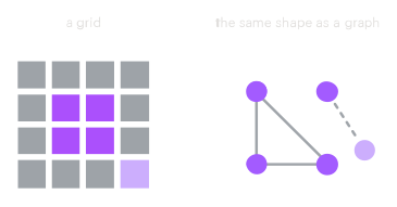
Apply the model to the site’s exercise. A grid is a graph: each cell is a node, and each cell has edges to its orthogonal neighbors (up, down, left, right - the exercise’s “not diagonally” is precisely the edge definition). An island is a connected component: a maximal set of land nodes where every node can reach every other node by walking along edges. Counting islands means counting connected components. The algorithm is BFS wearing a different hat:

• Scan the grid. The first time you find an unvisited land cell, you have found a new island - start a BFS (or depth-first search; either works for components) from it, marking every cell it reaches as visited.
• The search floods across the island through the land edges and stops at the water. Every cell it touched is now visited, so the scan will never count them again.
• The next unvisited land cell starts the next island. The number of starts is the answer.

This is the flood fill pattern - the algorithm that fills a connected region in a paint program, and the one that a “does this network have a path” question reduces to. The visited set is the crux: without it, the flood would recirculate forever across the same land cells; with it, each cell is touched exactly once, and the whole scan costs $O(V + E)$ for the grid. The grid-specific trick is just BFS with the modeling step done for you.

The BEAM is a graph

The site’s Process Ring exercise uses the same idea in a different medium. Spawn $n$ processes wired into a ring - each process knows its successor - and pass a token around. That is a graph with a specific name: a cycle, the simplest connected graph there is, with $n$ nodes and $n$ edges. The token is a message hopping along edges; the BEAM’s per-process mailboxes are the edges; and the exercise’s point - that message passing is the fundamental operation - is the point here too. A graph is not something you draw; it is something you traverse. On the BEAM, traversal is literally a message sent from one node to the next.

The connection goes beyond the exercise. The site’s dining developers article is a deadlock story, and deadlock is a graph property: build the wait-for graph, where an edge from A to B means “A is waiting for B,” and a deadlock is exactly a cycle in that graph - a ring of processes, each waiting for the one ahead of it, none able to move. The What the BEAM actually is article describes a runtime whose scheduler is itself a graph algorithm - a work-stealing scheduler is a graph of runnable processes with idle schedulers stealing work across edges. When the project says the BEAM is a broker and the broker is the message bus, it is making the same point from the other side: the runtime is a graph, and every piece of it - mailbox, supervisor tree, scheduler - is graph machinery wearing runtime clothes.

When the hops cost: Dijkstra

BFS answers “shortest path” when every hop costs the same. Add weights - the road is 5 miles, the other is 12 - and BFS is no longer correct, because the fewest hops is not necessarily the cheapest route. The weighted sequel is Dijkstra’s algorithm (a chapter of its own in the algorithms introduction, the 9th in the second edition): repeatedly take the unvisited node with the smallest known total distance, relax its edges, and record better paths when you find them. The search shape stays the same: a frontier expands outward from the source. Replace the queue with a priority structure that always expands the cheapest frontier node first.

Dijkstra is where greedy thinking and graph thinking meet. At every step it commits to the closest unvisited node, and the algorithm works because edge weights are non-negative, so no later discovery can offer a cheaper route to a node that was already settled. That greedy commitment is the subject this site will treat elsewhere; here, remember the split - BFS for unweighted graphs, Dijkstra for weighted ones. Both “expand the frontier” search, differing only in what the frontier is sorted by.

Where to go next

• Number of Islands - connected components in a grid, the exercise this article is built around.
• Process Ring - the cycle graph on the BEAM: message passing as graph traversal.
• Print in Order - topological sort: a valid order, or a cycle (deadlock) and an empty list.
• Dining Philosophers - the wait-for cycle as an exercise, the same deadlock this article names.
• The dining developers - deadlock as a cycle in the wait-for graph.
• Binary trees: where the log in O(log n) lives
  • the tree is a graph that forbids cycles; the shapes the log lives in.
• Stacks, queues, and associative arrays
  • the queue that makes BFS breadth-first.
• Recursion - the depth-first twin of BFS, and the visited set that keeps both finite.
• What the BEAM actually is and The BEAM is the broker - the runtime whose scheduler and mailboxes are graph machinery.
• Dijkstra’s algorithm: when every hop costs something
  • the weighted sequel this article promised: BFS’s frontier, sorted by cost instead of hops.

Graphs model how things are connected to one another. The payoff is that “connected” stops being vague and becomes an algorithm. An island is a connected component. A ring of processes is a cycle. A deadlock is a cycle in the wait-for graph. Each example uses the same two-part move from the introduction: model the problem as a graph, then run the search. The grid, the BEAM, and the dinner table were graphs already. Point the algorithm at them.