The first lesson in every algorithm course is the sentence people repeat forever: “hash tables are O(1).” It is true. It explains why Contains Duplicate, Two Sum, and Group Anagrams belong to “arrays and hashing.” It is also - read carefully - a half-truth. The fine print is where the skill lives. A hash table’s lookup is O(1) on average. That average depends on two design decisions every working programmer should be able to name. They separate a hash table from a very slow array in disguise. This article covers the superpower, the fine print, and what both mean for the exercises the site grades.
The superpower
The data-structures text introduces the hash table with deserved enthusiasm: “Most programming languages include a data structure called a hash table, and it has an amazing superpower: fast reading.” The same chapter gives the promise with its qualifier intact: “Looking up a value in a hash table has an efficiency of O(1) on average, as it usually takes just one step.”wengrow In Python they are dictionaries. In JavaScript they are objects and Maps. In Elixir they are maps. One structure, many names. The site’s associative-arrays article is where those names meet. This article explains what sits underneath them.
A hash table is an array plus a hash function. The hash function takes a key - any key, a string, a number, a tuple - and computes an array index. To store “french fries costs 75 cents,” run “french fries” through the hash function, get a slot number, and put the price there. To look it up, run “french fries” through the same function and go straight to that slot. No scanning. No searching. No comparison against the other keys. The key tells you where its value lives. That is the superpower. It turns “did I see this value before” from a scan over everything seen so far (O(n)) into a single lookup (O(1)). The site’s exercises use exactly this idea: Contains Duplicate asks “have I seen this number before?” n times, and Two Sum asks the same question with a subtraction - “have I seen target - x before?” - which the next section shows in code.
The first fine print: collisions
The hash function turns a key into a slot. It cannot guarantee that different keys get different slots. There are far more possible keys than slots - hashing compresses a huge key space into a small array - so two keys will sometimes land in the same cell. The data-structures text defines the failure mode precisely:
Trying to add data to a cell that is already filled is known as a collision. Fortunately, there are ways around it.
The standard solution is separate chaining: “when a collision occurs, instead of placing a single value in the cell, it places in it a reference to an array.”wengrow The cell becomes a bucket. The bucket holds every key that hashed there. A lookup that lands in that bucket must scan it to find its key. That scan is the fine print. A hash table with one bucket per cell and one key per bucket does O(1) lookups - one step, always. A hash table where everything collides into one bucket does O(n) lookups - a linear scan of the whole pile. That is exactly the site’s algorithms-past-the-interview warning: teams “discover at 3 a.m. that their ‘O(1) lookup’ was a linear scan in disguise.”
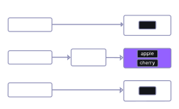
The text states the lesson directly: “it’s critical that a hash table is designed in such a way that it will have few collisions and, therefore, typically perform lookups in O(1) time rather than O(N) time.” Few collisions are a design goal, not a property of the concept. The hash function provides them: “a good hash function, therefore, is one that distributes its data across all available cells. The more we can spread out our data, the fewer collisions we’ll have.”
The second fine print: load factor and resizing
A good hash function spreads the data, but it needs room to spread into. The load factor measures how full the table is. The algorithms introduction defines it in one line: “The load factor of a hash table is easy to calculate. Hash tables use an array for storage, so you count the number of occupied slots in an array. For example, this hash table has a load factor of 2/5, or 0.4.” The same chapter gives two requirements for a fast hash table: “a low load factor” and “a good hash function.” The load factor is the space parameter. More slots means fewer collisions and faster lookups. The cost is memory: a table with mostly empty slots wastes it.
The engineering solution is resizing: when the load factor crosses a threshold (commonly 0.7 or 0.75), grow the array and reinsert every key, recomputing its hash in the new, larger table. Resizing is expensive. It touches every element. This is where the second half of the O(1) claim needs its qualifier. The resize does not happen often, and when it does, the table doubles. The elements moved by successive resizes form the sum 1 + 2 + 4 + … which stays below the total number of inserts. The occasional expensive step is paid for by the cheap ones around it, so the average cost per insert stays O(1). The site’s Queue with Two Stacks exercise uses the same amortized argument: every operation is cheap except the rare one that shuffles everything, and that shuffle is spread across the average. O(1) on average means O(1) per operation over a long sequence, not O(1) on every single operation.
What the map actually is
The textbook picture - array, hash function, resize at 0.75 - is the one the
fine print above is about. It is not the picture inside every runtime. Two
maps you will actually type, Elixir’s Map and a JavaScript object, both
promise O(1) lookup and both skip that picture for small sizes.
Erlang and Elixir maps switch representation at a small-size cutoff. Below about 32 keys, a map is a flat tuple of key/value pairs. Lookup is a short scan. That is O(n) with a tiny n, and it is faster than hashing for a handful of keys. Past that cutoff the map becomes a HAMT (hash array mapped trie): the hash bits pick a path through a tree of small arrays. There is no “double the whole table and reinsert.” A new key copies one path of the tree. The O(1) claim still holds in the usual sense - depth grows with the hash, not with n - but the expensive-resize story is a different machine.beam-maps
A typical JavaScript engine (V8) takes a different shortcut. Objects whose
keys arrive in a stable order get a hidden class: each key is a fixed
offset, and a lookup is not a hash at all. Add enough keys, delete keys, or
treat the object as a bag of arbitrary strings, and the engine falls back to
a real hash table. Map is that hash table from the first insert.
Hidden-class objects are why obj.x is fast; treating the object as a bag of
keys is why “I used an object as a hash table and it got slow” happens.v8-properties
The thesis does not change. Lookup is O(1) on average, and that average depends on representation, hash quality, and load. The BEAM’s small-map scan and V8’s hidden class both win the small-n case without hashing. The HAMT and the JS hash table both keep the large-n case from becoming a linear scan. The 3 a.m. failure mode is still the same: collisions (or that fallback) turning an O(1) lookup into an O(n) walk.
Why the exercises are hashing problems
Once you understand the mechanism, the site’s “arrays and hashing” exercises share one design skill: choosing the key.
Contains Duplicate is the seed: walk the list, check “have I seen this before?” in a set, and insert what you have not seen. That is one lookup per element and O(n) total. A nested scan would be O(n^2) - the quadratic cliff from the sorting article - so turn the “seen” list into a “seen” table.
Two Sum uses the same structure with the question flipped. For each number x, look for target - x - the complement. If you have seen it, you have the answer. In Elixir the whole algorithm is the reduce_while from the site’s own exercise, and it runs exactly as written:
defmodule TwoSum do
  def find(nums, target) do
    {_, _, found} =
      Enum.reduce_while(nums, {%{}, 0, nil}, fn x, {seen, i, acc} ->
        case Map.fetch(seen, target - x) do
          {:ok, j} -> {:halt, {seen, i, {j, i}}}
          :error -> {:cont, {Map.put(seen, x, i), i + 1, acc}}
        end
      end)

    found
  end
end
TwoSum.find([2, 7, 11, 15], 9) returns {0, 1}, and TwoSum.find([3, 2, 4], 6) returns {1, 2}. The complement map is the whole trick. The map is the hash table.
Group Anagrams makes key design the problem itself. Two words are anagrams when they use the same letters in different orders - “eat” and “tea” are the same multiset of letters. Give every anagram group a key that is the same for all of them: sort the letters (“eat” and “tea” both become “aet”) or count them into a fixed-shape histogram. The sorted-letter key takes the sorting article’s idea and puts it in a hash function’s clothes. The sorting is not the point; the key it produces is. The map from key to group is the O(1) lookup doing its job. The category’s fourth member, Product of Array Except Self, is the honest exception: same category, different technique (prefix products, no hashing at all). The category name is a filing convention, not an algorithm.
The fine print in the wild
The average-case caveat matters in production. A hash function that spreads normal keys well can be forced into collisions: feed a hash table keys that all hash to the same slot. That is easy to construct when the hash function is public and simple. Every lookup then becomes a linear scan, turning an O(1) data structure into an O(n) one while the code itself looks unchanged. This is the hash flooding class of denial-of-service attacks.crosby-wallach Real web frameworks have been hit by attacker-controlled keys (form fields, JSON keys) that collide catastrophically. The production countermeasure applies the same fine print defensively: use randomized hash seeds and cryptographic hashes for untrusted keys, so the attacker cannot predict the collisions. When someone tells you a hash table is O(1), ask: whose keys, and which hash function?
The advanced relative: Bloom filters
The fine print has a famous sequel. A Bloom filter is a hash-table cousin with a different trade: it answers “have I seen this before?” with a tiny, fixed memory footprint, at the price of a bounded error rate. The advanced data-structures reference states the trade in its title: “Bloom filter: As fast as hash tables, but saves memory (with a catch),” and names the inventor: “a data structure named after Burton Howard Bloom, who invented them in the 1970s.” The catch is the false positive. A Bloom filter can say “maybe seen” when it has not seen the item, but it never says “definitely not seen” when it has.bloom-1970 That asymmetry fits structures that must not miss. The site’s algorithms-past-the-interview names the production use - a dedupe layer that trades “a bounded false-positive rate for constant memory.” In the Bloom filter, the hash table’s fine print becomes a feature.
Where to go next
- Contains Duplicate - the seen-set seed: O(1) lookups where a nested scan would be O(n^2).
- Two Sum - the complement map, in four languages.
- Group Anagrams - key design as the actual problem: one key per anagram class.
-
Stacks, queues, and associative arrays
- the associative array’s other names and jobs.
-
Sorting: the wall at n log n
- the sorted-letter key, and the quadratic cliff hashing avoids.
- Queue with Two Stacks - the amortized argument that makes the occasional resize free on average.
- What O(n) actually promises - the shape of the growth, average case included.
-
Algorithms past the interview
- the “O(1) lookup that was a linear scan in disguise,” and the Bloom filter in production.
Hash tables are O(1) on average. That average is earned by a hash function that spreads, a load factor with room to spread into, and amortized accounting that pays for the rare resize with the cheap operations around it. Forget one of the three and O(1) quietly becomes O(n), a linear scan wearing a data structure’s clothes. Remember all three and the exercises make sense: every “have I seen this before” becomes a lookup, every complement becomes a map entry, and every anagram class becomes a key. The superpower is real. The fine print makes it real.
-
↩
Jay Wengrow, A Common-Sense Guide to Data Structures and Algorithms, 2nd ed., Pragmatic Bookshelf, 2020 - the hash-table chapter is the source of the “amazing superpower: fast reading” framing, the O(1)-on-average promise, and the separate-chaining treatment of collisions quoted above.
-
↩
Erlang/OTP Efficiency Guide (“Advanced” chapter, erlang.org) - the switch between small maps (up to 32 keys) and large maps backed by the HAMT structure.
-
↩
Camillo Bruni, “Fast properties in V8,” V8 blog, August 2017 - hidden classes give objects with a stable key order fixed-offset property access; objects fall back to slow dictionary-mode properties when keys are too dynamic.
-
↩
Scott A. Crosby and Dan S. Wallach, “Denial of Service via Algorithmic Complexity Attacks,” Proceedings of the 12th USENIX Security Symposium, 2003 - adversarial hash collisions as a low-bandwidth DoS, and randomized hashing as the defense.
-
↩
Burton H. Bloom, “Space/Time Trade-offs in Hash Coding with Allowable Errors,” Communications of the ACM 13(7), 1970 - the Bloom filter: bounded false positives, no false negatives, in fixed memory.