Binary trees: where the log in O(log n) lives

Every structure in the previous article was a line. Arrays, stacks, queues, and associative arrays all arrange their data in a row - even the associative array, which jumps straight to a slot, stores the slots in a row. A tree is the first shape that forks. One node points at two more, each of those points at two more, and the number of nodes you can reach doubles at every step down. That doubling is why trees matter: it is where the “log” in $O(\log n)$ lives. The site’s tree problem, Validate Binary Search Tree, is the payoff - a binary tree with an ordering rule, and a check you have to get exactly right. This article covers the shape underneath it. If the $O(\log n)$ notation is new, read What O(n) actually promises first.

What a binary tree is

A tree is built from nodes and edges. One node is the root, where everything starts. Every node can have children, and the nodes with no children are leaves. A binary tree adds one rule: no node gets more than two children. The textbook definition is direct:

A binary tree is a special type of tree where nodes can have at most two children (hence the name binary, meaning two). These are traditionally called left child and right child.

The “left” and “right” labels matter. An ancestry tree makes that clear: “everyone has two biological parents.” Your parents, grandparents, and great-grandparents form levels, and the two parents occupy fixed sides. The other algorithms textbook says it directly: “in a degree 2 tree, which is usually called a binary tree, each node can have at most two children.” Degree two. Two branches, no more.

The site’s own problem relies on two details. First, an empty child is a real thing, not an absence: a node can have a left child and no right child, or neither. In the problem’s input format, the empty child is spelled #, and a node is written as its value followed by its two subtree strings:

"5,3,#,#,7,#,#"    # 5, whose left child is 3 (with no children) and whose
                   # right child is 7 (with no children)

Second, every node is the root of its own subtree. The right child of the root is also the root of a smaller tree, with its own children and grandchildren. A binary tree is a node with two binary trees attached. That description applies again to each smaller tree. This self-similarity is the subject of the next two sections.

Why binary? Where the log comes from

The rule says at most two children. Why two, rather than three, one, or seventeen? The answer is the doubling argument. It is the key fact about binary trees.

Imagine a tree where every level is as full as possible. The root is one node. Its two children make the second level. Each child has two children, so the third level holds four. The fourth holds eight, and the fifth holds sixteen. As the algorithms book puts it: “each time we add a new full level to the tree, we end up roughly doubling the number of nodes that the tree has. (Really, we’re doubling the nodes and adding one.)”

That is where the log comes from. A tree of height $H$ - $H$ levels of nodes - holds up to $2^H$ nodes. Reverse that: to hold $N$ nodes, a balanced binary tree needs about $\log_2 N$ levels. The reference book states both directions: “a full complete binary tree of height H has $2^H$ nodes. To look at it from the other direction, a full complete binary tree that contains N nodes has height $\log_2(N)$.”

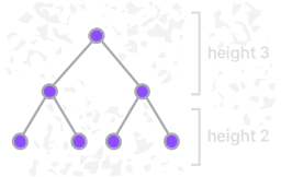
Here is the “why two” answer. Each level doubles capacity, so reaching a particular node takes at most one step per level. The number of levels grows as the log of the number of nodes. A tree with a thousand nodes has about ten levels. A tree with a million nodes has about twenty. Adding a level multiplies capacity, so capacity grows exponentially while height grows logarithmically. Binary search uses the same trade when it eliminates half of the remaining data per step. Two is the smallest branching factor that still doubles. One child per node is a chain - a list wearing a tree costume, with $N$ levels for $N$ nodes and no log in sight. Three children would triple instead of doubling, but the log base barely changes ($\log_3 N$ vs $\log_2 N$ is a constant factor), while the bookkeeping triples. Two is the sweet spot: the minimum that makes height logarithmic, with the cheapest branching. The “log” in $O(\log n)$ lives in the tree’s levels, because the tree forks in two.

The structure recursion was made for

The site’s recursion article defines recursion the usual way: a function calls itself, and a base case stops it. Trees make that definition useful rather than clever. A tree is a recursive definition in diagram form. A binary tree is empty, or a value with a left binary tree and a right binary tree. That sentence is already an algorithm.

The algorithms literature explains why: “recursion is key when dealing with data structures that have an arbitrary number of levels of depth. A tree is such a data structure, as it can have an infinite number of levels.” A loop would have to track a stack of “come back here later” bookmarks by hand. Recursion lets the call stack - the subject of that article - hold those bookmarks for you, one frame per level.

The Elixir representation makes the recursion literal, and it matches the shape used by the site’s problem:

@type tree :: :empty | {:node, integer(), tree(), tree()}

def depth(:empty), do: 0
def depth({:node, _value, left, right}), do: 1 + max(depth(left), depth(right))

def size(:empty), do: 0
def size({:node, _value, left, right}), do: 1 + size(left) + size(right)

Read depth the way the induction article teaches. The :empty clause is the base case: an empty tree has depth zero. The {:node, ...} clause is the step: the depth of a tree is one plus the depth of its deeper subtree. That phrase means the same function runs on a smaller tree; this is the induction hypothesis doing its job. The tree contains its own base case (empty) and recursive step (the two children). That is why recursive functions over trees are usually three or four lines: match the empty tree, match a node, and combine the two recursive calls. The code follows the definition. Both follow the data.

Traversals: three orders, one recursion

A tree is recursive, so “visit every node” means “visit me, then visit my subtrees.” The three classic traversals put the “visit me” step in three different places. The reference book defines the first one plainly: “In a preorder traversal, the algorithm processes a node, and then its left child, and then its right child.” The other two move the node:

• Preorder: node, left, right.
• Inorder: left, node, right.
• Postorder: left, right, node.

Each uses the same three-line recursion. Only the position of the “process” line changes:

def preorder(:empty), do: []
def preorder({:node, value, left, right}), do: [value | preorder(left) ++ preorder(right)]

def inorder(:empty), do: []
def inorder({:node, value, left, right}), do: inorder(left) ++ [value | inorder(right)]

def postorder(:empty), do: []
def postorder({:node, value, left, right}), do: postorder(left) ++ postorder(right) ++ [value]

The names tell you the order: pre (before), in (in between), post (after) - before, between, or after the children. These orders have direct uses. Preorder is the wire format: a node, then its left subtree, then its right subtree is exactly the string the site’s problem hands you, "5,3,#,#,7,#,#", with # as the empty tree. Rebuild the tree with a recursive descent that reads a node, builds the left subtree, builds the right subtree, and stops at #. Inorder has the classic fact attached: on a binary search tree, an inorder traversal visits values in sorted order, because left descendants are smaller and right descendants are larger. Postorder is what you use when children must be processed before parents - deleting a tree (delete the children first), or computing a value that depends on the whole subtree below. Three orders. Three jobs.

The binary search tree: order in the levels

A binary search tree is a binary tree with a global ordering rule. That rule is the point of the site’s problem:

A binary search tree is a binary tree that also abides by the following rules: Each node can have at most one left child and one right child. A node’s left descendants can only contain values that are less than the node itself. Likewise, a node’s right descendants can only contain values that are greater than the node itself.

The important word is descendants, not children. Immediate children are not enough; every value in the left subtree must be smaller, and every value in the right subtree must be greater. The rule applies recursively at every node. The site’s problem description says why: “the rule must hold for every descendant, not only for immediate children.” This is the classic BST bug, and the problem makes you confront it. Consider a tree whose root is 5, with a left child 3, and the 3 has a right child 6. Locally, every parent-child pair is fine: 5 > 3 and 3 < 6. But 6 is in the left subtree of 5, where every value must be less than 5. The tree is not a BST. Checking only immediate children would incorrectly accept it. The correct check passes the allowed range down the recursion: each node must be greater than every ancestor to its left and less than every ancestor to its right. Pass the current lower and upper bounds into the recursive calls.

Searching in a BST turns doubling into a procedure. Start at the root. If the value you want is smaller, it can only be in the left subtree; if larger, only in the right. “Each step eliminates half of the remaining nodes from our search,” as the algorithms book walks through, “which is the apt description for any algorithm that eliminates half of the remaining values with each step” - so search is $O(\log n)$ on a balanced tree. That matches binary search in a sorted array. The same textbook explains why the structure exists: “Where binary search trees really shine over ordered arrays, though, is with insertion.” An ordered array inserts in $O(n)$ - everything after the insertion point shifts. A BST inserts in $O(\log n)$ - one walk down the levels, one new leaf. The caveat matters: the log only holds for a balanced tree. Insert values in sorted order and the “tree” becomes a chain - one child per node - and search degrades to $O(n)$. The shape delivers its promise only when the levels stay full enough to keep doubling, which is why real systems use self-balancing variants. The tree earns the log by staying a tree.

The tree hiding in the array

The shape appears in one more place, and it connects the tree to the structures from the previous article. A complete binary tree - every level full except possibly the last, filled left to right - needs no pointers. The reference book gives the recipe: “You can easily store a complete binary tree in an array using a simple formula. Start by placing the root node at index 0. Then, for any node with index i, place its children at indices $2 \times i + 1$ and $2 \times i + 2$.”

That formula puts a heap - a complete binary tree where every node’s value is at least as large as its children’s - in a plain array. No node structs. No pointers. Just index arithmetic. The priority queue, the scheduler that always hands you the largest (or smallest) item in $O(\log n)$, is a tree in an array’s clothing. The lesson matches the one the stacks-and-queues article drew: the shape of a structure is a discipline, not a layout. A queue is a discipline applied to an array; a heap is a tree applied to an array; and a binary search tree is a tree with an ordering discipline applied on top. The shape is the fork, the two children, and the levels that double. Storage and guarantees come after that.

Where to go next

• Validate Binary Search Tree on /problems - the article’s ideas as an actual exercise, in Elixir, Erlang, TypeScript, or Lua: parse the preorder string, build the tree, and enforce the descendant rule with range-checking recursion.
• Maximum Tree Depth - the other half of the recursive walk: consume the same preorder string and return the number of levels in the longest root-to-leaf path, without building a node structure at all.
• Recursion: the pattern that calls itself
  • the call stack is the machinery that lets a recursive tree function hold its place in each subtree.
• Induction: the proof pattern recursion already uses
  • why “assume the smaller subtrees, combine the results” is a proof, not just a shortcut.
• What O(n) actually promises - the notation behind the doubling argument, and the balanced-vs-degenerate caveat that decides whether the log actually shows up.
• Stacks, queues, and associative arrays
  • the linear structures this article’s tree forked away from, and the heap that puts a tree back inside an array.
• Sorting: the wall at n log n - the merge tree is this tree wearing a sorting hat, and the log in $O(n \log n)$ is this log.
• Graphs: when the answer is a hop away
  • a tree is a graph that forbids cycles; this article’s shapes are the graph’s first special case.
• Dijkstra’s algorithm: when every hop costs something
  • the heap that puts a tree back inside an array is the frontier of the algorithm that made the heap famous.

A binary tree is a value, two subtrees, and a rule about how many. Two children is the smallest fork that still doubles capacity at every level. That doubling is where the log in $O(\log n)$ lives. The tree defines itself recursively - empty, or a value with two smaller trees - so the code that walks it follows the same pattern: handle the empty tree, handle the node, combine the two recursive calls. That is why the site’s tree problems are checks and walks, not constructions. Recursion constructs the shape. The shape is the data. The remaining job is enforcing the rule for every descendant, not just the children you can see.